Table of Contents
Introduction to Cramer’s Rule


Cramer’s rule is an effective approach for solving linear equation systems using determinants and matrices. Cramer’s rule gives a formula for finding the unique solution for each variable in a square and non-singular coefficient matrix. The approach includes determining the determinants of modified matrices in which the coefficient column of each variable is replaced by the constant column. Cramer’s rule is an elegant solution for small systems, but it becomes computationally expensive for larger ones owing to repeated determinant computations. Nonetheless, it is a valuable tool in linear algebra, offering insight into the solvability and uniqueness of solutions in linear systems.
Definition of Cramer’s Rule
Cramer’s Rule is a method for solving a system of linear equations in which the answer for each variable is expressed as a ratio of two determinants. It is applicable to square and non-singular coefficient matrices, and it provides unique solutions for the system’s variables.


Procedure and formula in Cramer’s rule:
Cramer’s Rule is a mathematical technique used to find the solutions of a system of linear equations with the same number of equations as variables. Given a system of linear equations in the form of:
a₁₁x + a₁₂y + a₁₃z + … + a₁ₙu = b₁
a₂₁x + a₂₂y + a₂₃z + … + a₂ₙu = b₂
a₃₁x + a₃₂y + a₃₃z + … + a₃ₙu = b₃
…
aₘ₁x + aₘ₂y + aₘ₃z + … + aₘₙu = bₘ
where ‘x’, ‘y’, ‘z’, …, ‘u’ are the variables to be solved for, ‘aᵢⱼ’ are the coefficients, and ‘bᵢ’ are constants, Cramer’s Rule states that the solution for each variable can be expressed as a ratio of two determinants.
For the ‘i’-th variable ‘xᵢ’, the solution is given by:
xᵢ = det (Aᵢ) / det(A)
where ‘det(A)’ is the determinant of the coefficient matrix of the system, and ‘det (Aᵢ)’ is the determinant obtained by replacing the ‘i’-th column of ‘A’ with the column matrix of constants ‘b₁, b₂, …, bₘ’.
Cramer’s Rule is applicable only when the coefficient matrix ‘A’ is square and non-singular, meaning it has a non-zero determinant.
Cramer’s Rule for 2by2 matrix
Cramer’s Rule can be explained using a general 2×2 matrix. Consider a system of linear equations with two variables ‘x’ and ‘y’, represented as:
a₁₁x + a₁₂y = b₁
a₂₁x + a₂₂y = b₂
To apply Cramer’s Rule, we first calculate the determinant ‘D’ of the coefficient matrix ‘A’
D = (a₁₁ * a₂₂) – (a₁₂ * a₂₁)
Then, we create two modified matrices ‘A₁’ and ‘A₂’:
A₁ is obtained by replacing the first column of ‘A’ with the column matrix of constants (b₁, b₂):
A₂ is obtained by replacing the second column of ‘A’ with the column matrix of constants (b₁, b₂):
Next, we calculate the determinants of ‘A₁’ and ‘A₂’:
D₁ = (b₁ * a₂₂) – (a₂₁ * b₂)
D₂ = (a₁₁ * b₂) – (b₁ * a₂₁)
Finally, we find the solutions for ‘x’ and ‘y’ using Cramer’s Rule:
x = D₁ / D
y = D₂ / D
If the determinant ‘D’ is non-zero, the system has a unique solution. If ‘D’ is zero, the system may have no solution or infinitely many solutions. Cramer’s Rule provides a concise way to find solutions for small systems of linear equations.
Cramer’s rule for 3 by 3 matrix
Cramer’s Rule can be explained using a general 3×3 matrix for a system of three linear equations with three variables ‘x’, ‘y’, and ‘z’, represented as:
a₁₁x + a₁₂y + a₁₃z = b₁
a₂₁x + a₂₂y + a₂₃z = b₂
a₃₁x + a₃₂y + a₃₃z = b₃
To apply Cramer’s Rule, we first calculate the determinant ‘D’ of the coefficient matrix ‘A’:
D = a₁₁(a₂₂a₃₃ – a₂₃a₃₂) – a₁₂(a₂₁a₃₃ – a₂₃a₃₁) + a₁₃(a₂₁a₃₂ – a₂₂a₃₁)
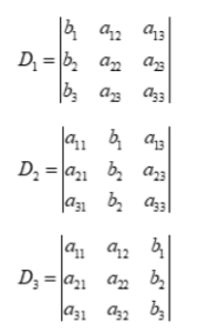
Next, we create three modified matrices ‘A₁’, ‘A₂’, and ‘A₃’:
A₁ is obtained by replacing the first column of ‘A’ with the column matrix of constants (b₁, b₂, b₃):
A₂ is obtained by replacing the second column of ‘A’ with the column matrix of constants
A₃ is obtained by replacing the third column of ‘A’ with the column matrix of constants (b₁, b₂, b₃):
Next, we calculate the determinants of ‘A₁’, ‘A₂’, and ‘A₃’:
Finally, we find the solutions for ‘x’, ‘y’, and ‘z’ using Cramer’s Rule:
x = D₁ / D
y = D₂ / D
z = D₃ / D
If the determinant ‘D’ is non-zero, the system has a unique solution. If ‘D’ is zero, the system may have no solution or infinitely many solutions. Cramer’s Rule provides a method to find solutions for small systems of linear equations, but it becomes computationally expensive for larger systems.


Solved example in Cramer’s rule.
Let’s solve an example using Cramer’s Rule to find the solutions for a system of linear equations.
Consider the following system of linear equations:
2x + y – z = 5
x – 3y + 2z = -4
3x + 2y – 5z = 7
Solution: Solution using Cramer’s Rule:
Step 1: Calculate the determinant ‘D’ of the coefficient matrix ‘A’:
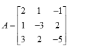
The determinant of the above matrix is
D = 2(-3(-5) – 2(2)) – 1(1(-5) – 2(3)) – (-1)(1(2) – (-3)(3))
D = 2(-15 – 4) – 1(-5 – 6) – (-1)(2 + 9)
D = 22 + 11 – 11
D = 22
Step 2: Create the modified matrices ‘A₁’, ‘A₂’, and ‘A₃’:
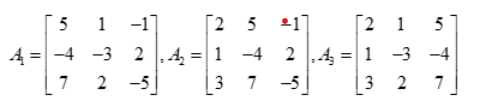
Step 3: Calculate the determinants ‘D₁’, ‘D₂’, and ‘D₃’:
D₁ = 5(-3(-5) – 2(2)) – 1(-4(-5) – 2(7)) + (-1)(-4(2) – (-3)(7))
D₁ = 5(15 – 4) – 1(20 – 14) + (-1)(-8 + 21)
D₁ = 55 – 6 -13
D₁ = 36
D₂ = 2(-4(-5) – 2(7)) – 5(1(-5) – 2(3)) – (-1)(1(7) – (-4)(3))
D₂ = 2(20 – 14) – 5(-5 – 6) – (-1)(7 + 12)
D₂ = 12 + 55 – 19
D₂ = 48
D₃ = 2(-3(7) – 2(-4)) – 1(1(7) – (-3)(4)) – 5(1(2) – (-3)(3))
D₃ = 2(-21 +8) – 1(7 + 12) – 5(2 + 9)
D₃ = -26 – 19 + 55
D₃ = 10
Step 4: Find the solutions for ‘x’, ‘y’, and ‘z’ using Cramer’s Rule:
x = D₁ / D = 36 / 22 = 18/11
y = D₂ / D = 48 / 22 = 24/11
z = D₃ / D = 10 / 22 = 5/11
So, the solutions for the given system of linear equations are:
x = 18/11, y = 24/11, and z = 5/11.
Limitations in Cramer’s rule
- Cramer’s Rule is a useful method for solving small systems of linear equations. However, it has some limitations that make it less practical for larger systems or certain cases :
- Computational Complexity: Cramer’s Rule involves computing determinants, which can be computationally expensive, especially for larger matrices. As the size of the system increases, the time and resources required for calculating determinants become prohibitive.
- Non-Applicability to Singular Matrices: Cramer’s Rule requires that the coefficient matrix is square and non-singular (i.e., its determinant is non-zero). If the determinant of the matrix is zero, the rule cannot be applied, and the system might have either no solution or infinitely many solutions.
- Numerical Instability: When solving systems with matrices that have extremely small or large determinants, Cramer’s Rule may suffer from numerical instability and produce inaccurate results due to limited precision in floating-point arithmetic.
- Inefficient for Large Systems: For large systems of equations, the computational effort and memory requirements to find determinants and create modified matrices become excessive, making the method impractical.
- Division by Determinant: Cramer’s Rule involves dividing determinants to find the solutions, and if the determinant is very close to zero (nearly singular), this can lead to significant errors in the solutions.
- No Shortcuts for Repeated Calculations: In certain applications, such as solving a system with the same coefficient matrix but different constant vectors, Cramer’s Rule requires repeating the entire process for each new constant vector, further increasing computational overhead.
- Given these limitations, for larger systems or situations where efficiency and numerical stability are crucial, other methods like matrix factorization (e.g., LU decomposition, Gaussian elimination) or iterative solvers are often preferred over Cramer’s Rule. These alternative methods can handle a broader range of problem sizes and offer better numerical stability and efficiency.
Frequently asked questions on Cramer’s Rule
What is Cramer’s rule in the matrix?
Cramer's Rule is a method used to solve systems of linear equations represented in matrix form. It provides a formula to find the unique solutions for each variable by using determinants and modified matrices. The rule is applicable for square and non-singular coefficient matrices.
What is Cramer’s Rule also known as?
Cramer's Rule is also known as the Cramer's method or Cramer's determinants.
Does Cramer’s Rule always work?
No, Cramer's Rule is not always applicable. It only works with square and non-singular coefficient matrices. Cramer's Rule cannot be used if the determinant of the coefficient matrix is zero (a singular matrix), thus the system may have no unique solution or infinitely many solutions.
What is the limitation of Cramer’s Rule?
Cramer's Rule has limitations such as computational complexity for larger systems, inefficiency for repeated calculations, numerical instability for matrices with very small or large determinants, and inapplicability to singular matrices with zero determinant, resulting in either no solution or infinitely many solutions.
In what condition does Cramer’s Rule fail?
When the coefficient matrix of the system of linear equations is unique, meaning it has a determinant of zero, Cramer's Rule fails or is not applicable. Cramer's Rule cannot be utilised to discover a unique solution in such instances, and the system may have no solution or infinitely many solutions.
What is Cramer’s Rule formula?
Cramer's Rule formula for solving a system of linear equations with variables 'x', 'y', ..., 'u' is: x = det(A₁) / det(A), y = det(A₂) / det(A), ..., u = det(Aₙ) / det(A) where 'det(A)' is the determinant of the coefficient matrix 'A', and 'det(Aᵢ)' is the determinant obtained by replacing the 'i'-th column of 'A' with the column matrix of constants.
What is Cramer’s Rule for 3 equations?
Cramer's Rule for a system of three linear equations with three variables (x, y, and z) can be expressed as follows: Given the system of equations: a₁₁x + a₁₂y + a₁₃z = b₁ a₂₁x + a₂₂y + a₂₃z = b₂ a₃₁x + a₃₂y + a₃₃z = b₃ The solutions for x, y, and z are given by: x = det(A₁) / det(A) y = det(A₂) / det(A) z = det(A₃) / det(A) where: det(A) is the determinant of the coefficient matrix: det(A₁) is the determinant of the matrix obtained by replacing the first column of A with the column matrix of constants (b₁, b₂, b₃). det(A₂) is the determinant of the matrix obtained by replacing the second column of A with the column matrix of constants (b₁, b₂, b₃). det(A₃) is the determinant of the matrix obtained by replacing the third column of A with the column matrix of constants (b₁, b₂, b₃). Cramer's Rule provides a way to find unique solutions for x, y, and z in the system of three linear equations if the determinant det(A) is non-zero (i.e., the coefficient matrix is non-singular). If det(A) is zero, the system may have either no solution or infinitely many solutions, and Cramer's Rule cannot be applied.
Why is it called Cramer’s Rule?
Cramer's Rule is named after the Swiss mathematician and physicist Gabriel Cramer (1704-1752), who described the approach in his 1750 book Introduction alAnalyse des lignes Courbes Algébriques (Introduction to the Analysis of Algebraic Curves). Cramer investigated the use of determinants and matrices to solve systems of linear equations in this work, and the approach became known as Cramer's Rule in his honour. Cramer's work produced substantial advances to linear algebra, and his rule is still used in the area today.
What are the limitations of Cramer’s Rule?
Cramer's Rule has limitations, including computational complexity for large systems, inefficiency for repeated calculations, numerical instability for small/large determinants, inapplicability to singular matrices (zero determinant), and potential errors when dividing by determinants close to zero, making it unsuitable for larger systems and numerically sensitive cases.