Electrostatics: Concepts, Derivation & Examples
By Ankit Gupta
|
Updated on 10 Jul 2026, 12:28 IST
Electrostatics is where JEE physics stops feeling abstract. Every capacitor in a circuit, every spark of static on a dry winter day, and every photocopier in an office runs on the handful of laws packed into this chapter. It is also one of the most consistently rewarding chapters on the exam: the concepts build on each other in a strict, logical sequence — charge, force, field, potential, flux, capacitance — and a student who follows that sequence rarely gets caught off guard.
JEE Main and JEE Advanced typically draw 2–4 questions directly from electrostatics each year, and the chapter's ideas resurface constantly inside current electricity, magnetism, and even modern physics questions involving charged particles. Gauss's Law problems and capacitor networks are particular favourites of the examiners, because they reward students who understand symmetry rather than those who have simply memorised formulas.
Beyond the exam, electrostatics explains phenomena you interact with daily. Lightning is nature's demonstration of charge building up between clouds and ground until the electric field exceeds the breakdown strength of air. Capacitors store the electrostatic potential energy that powers camera flashes and smooths voltage in every phone charger. Photocopiers and laser printers rely on electrostatic charging and induction to transfer toner onto paper. This guide works through the chapter's laws, derivations, and problem-solving patterns in the order they're actually tested.
Coulomb's Law
Statement and Mathematical Formulation
Coulomb's Law states that the electrostatic force between two point charges is directly proportional to the product of their magnitudes and inversely proportional to the square of the distance between them, acting along the line joining them.
F = (1 / 4πε₀) × (q₁q₂ / r²) = k q₁q₂ / r²
Here, ε₀ is the permittivity of free space (8.85 × 10⁻¹² C²N⁻¹m⁻²), and k = 1/(4πε₀) ≈ 9 × 10⁹ N·m²/C² is the Coulomb constant. Like charges repel; unlike charges attract.
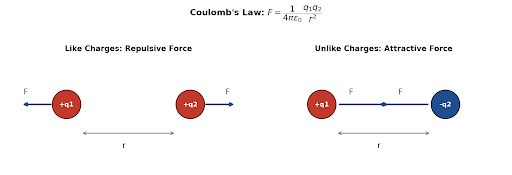
Figure 1: Coulomb's Law — force direction for like and unlike charge pairs.

Vector Form and the Superposition Principle
In vector form, the force on charge q₁ due to q₂, located at position vectors r₁ and r₂ respectively, is written using the unit vector r̂₁₂ pointing from q₂ to q₁:
F₁₂ = k (q₁q₂ / |r₁₂|²) r̂₁₂
Best Courses for You

JEE

NEET

Foundation JEE

Foundation NEET

CBSE
When more than two charges are present, the superposition principle applies: the net force on any charge is the vector sum of the individual Coulomb forces exerted by every other charge in the system, computed as if each pair existed in isolation.
F_net = F₁ + F₂ + F₃ + ... + Fₙ (vector sum)
Comparison with Gravitational Force
Coulomb's Law and Newton's Law of Gravitation share the same inverse-square structure, which is why students often confuse them. The key differences are worth knowing cold for conceptual JEE questions.
| Property | Electrostatic Force | Gravitational Force |
| Nature | Can be attractive or repulsive | Always attractive |
| Depends on | Product of charges, q₁q₂ | Product of masses, m₁m₂ |
| Constant | k ≈ 9 × 10⁹ N·m²/C² | G ≈ 6.67 × 10⁻¹¹ N·m²/kg² |
| Relative strength | Much stronger (for elementary particles, ~10³⁶ times gravity) | Extremely weak in comparison |
| Medium dependence | Depends on the medium (via permittivity) | Independent of medium |
Electric Field and Electric Field Lines
Definition of Electric Field Intensity
The electric field at a point is defined as the force experienced per unit positive test charge placed at that point, in the limit where the test charge is small enough not to disturb the source charges:
E = F / q₀ = kQ / r² (due to a point charge Q)
Electric field is a vector quantity, measured in N/C or equivalently V/m, and points in the direction a positive test charge would be pushed.
Electric Field for Different Charge Distributions
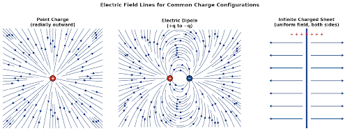
Figure 2: Electric field line patterns for a point charge, a dipole, and an infinite charged sheet.
Point charge: E = kQ/r², directed radially outward for positive Q and radially inward for negative Q.
Electric dipole: for a dipole of moment p = q(2a), the field at a point on the axial line (r ≫ a) is twice the field at an equatorial point at the same distance:
E_axial = 2kp / r³ E_equatorial = kp / r³
At a general point making angle θ with the dipole axis, the field magnitude is:
E = (kp / r³) √(3cos²θ + 1)
Charged ring (on its axis): for a ring of radius R carrying charge Q, the field at a point on the axis at distance x from the centre is:
E_ring = kQx / (x² + R²)^(3/2)
Notice that E_ring = 0 at the centre (x = 0), and the field is maximum at x = R/√2 — a result that occasionally appears directly in JEE questions.
Charged disc (on its axis): for a disc of radius R with uniform surface charge density σ, integrating contributions from concentric rings gives:
E_disc = (σ / 2ε₀) [1 − x / √(x² + R²)]
As R → ∞, this reduces exactly to the infinite-sheet result below — a useful check on the formula.
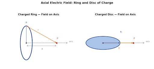
Figure 3: Geometry for the axial field of a charged ring and a charged disc.
Infinite sheet of charge: for a thin infinite sheet with uniform surface charge density σ, the field is uniform in magnitude and direction on each side, independent of distance from the sheet:
E_sheet = σ / 2ε₀
Properties of Electric Field Lines
- Field lines originate on positive charges and terminate on negative charges (or extend to infinity).
- Two field lines can never intersect — if they did, the field at that point would have two directions at once.
- The density of field lines in a region indicates the field's strength — closer lines mean a stronger field.
- Field lines are always perpendicular to the surface of a conductor in electrostatic equilibrium.
Electric Potential and Potential Difference
Definition and Relation with Electric Field
Electric potential at a point is the work done per unit positive charge in bringing a small test charge from infinity to that point, without any change in kinetic energy. It is a scalar quantity, measured in volts.
V = W / q₀ = kQ / r (due to a point charge Q)
Electric field and potential are related through a gradient relationship — the field points in the direction of steepest decrease of potential:
E = −dV/dr (or, in general, E = −∇V)
Equivalently, potential difference between two points equals the negative of the line integral of the electric field along any path connecting them:
V_B − V_A = −∫ₐᴮ E · dl
Potential Due to Various Charge Distributions
Point charge: V = kQ/r, a scalar that simply adds algebraically (not vectorially) when charges are combined — this makes potential calculations noticeably easier than field calculations.
Electric dipole: at a point making angle θ with the dipole axis (r ≫ a):
V = kp cosθ / r²
On the axial line (θ = 0°), V = kp/r²; on the equatorial line (θ = 90°), V = 0 even though the field there is not zero — a classic conceptual trap in MCQs.
Continuous charge distribution: found by summing (integrating) the contribution dV = k dq/r from every infinitesimal element of charge dq.
Equipotential Surfaces
An equipotential surface is a surface on which every point has the same electric potential. Two properties define how they behave:
- Equipotential surfaces are always perpendicular to electric field lines at every point of intersection.
- No work is done in moving a charge along an equipotential surface, since V is constant and W = qΔV = 0.
For a point charge, equipotential surfaces are concentric spheres centred on the charge; for a uniform field (like between capacitor plates), they are flat planes perpendicular to the field.
Gauss's Law
Statement and Mathematical Form
Gauss's Law relates the total electric flux through any closed surface to the net charge enclosed by that surface:
Φ_E = ∮ E · dA = Q_enc / ε₀
Its power lies in symmetry: for charge distributions with spherical, cylindrical, or planar symmetry, choosing a Gaussian surface that matches that symmetry lets you pull E outside the integral entirely, turning a difficult integration problem into simple algebra.
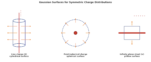
Figure 4: Gaussian surfaces chosen to match the symmetry of the charge distribution.
Applications
Infinite line charge (linear charge density λ): using a cylindrical Gaussian surface of radius r and length L coaxial with the wire, flux passes only through the curved surface:
E(2πrL) = λL/ε₀ ⇒ E = λ / (2πε₀r)
Uniformly charged solid sphere (total charge Q, radius R): using a spherical Gaussian surface of radius r:
Outside (r ≥ R): E = kQ/r² Inside (r < R): E = kQr/R³
Note the field grows linearly with r inside a uniformly charged sphere, peaks at the surface (E = kQ/R²), and then falls off as 1/r² outside — a graph JEE frequently asks students to sketch or interpret.
Infinite plane sheet (surface charge density σ): using a pillbox Gaussian surface straddling the sheet, with flux emerging through both flat faces:
E(2A) = σA/ε₀ ⇒ E = σ / 2ε₀
This matches the infinite-sheet result derived earlier from direct integration — Gauss's Law simply reaches the same answer far faster.
Capacitance and Capacitors
Parallel Plate Capacitor — Derivation
Consider two large, flat, parallel conducting plates of area A separated by a small distance d, carrying charges +Q and −Q. The field between the plates (superposing the fields of both sheets) is:
E = σ/ε₀ = Q / (Aε₀)
Since the plates are close together and the field is uniform, the potential difference is simply V = Ed:
V = Ed = Qd / (Aε₀)
Capacitance is defined as C = Q/V, so:
C₀ = ε₀A / d
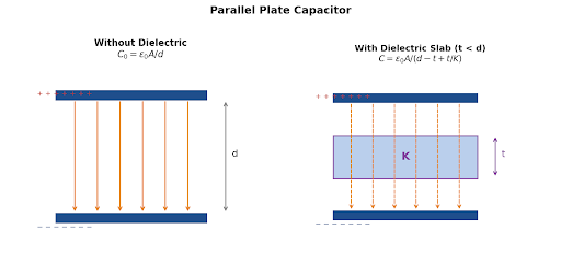
Figure 5: Parallel plate capacitor without and with a dielectric slab of thickness t.
Series and Parallel Combinations
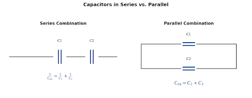
Figure 6: Capacitors in series share the same charge; capacitors in parallel share the same voltage.
In series, every capacitor carries the same charge Q, and the voltages add up, giving the reciprocal-sum rule:
1/C_eq = 1/C₁ + 1/C₂ + 1/C₃ + ...
In parallel, every capacitor has the same voltage V, and the charges add up directly:
C_eq = C₁ + C₂ + C₃ + ...
Energy Stored in a Capacitor
The energy stored equals the work done in charging the capacitor from 0 to Q, found by integrating the incremental work dW = (q/C)dq from 0 to Q:
U = ½CV² = Q²/2C = ½QV
Dielectrics and Their Effect on Capacitance
Inserting a dielectric of dielectric constant K (relative permittivity) between the plates reduces the effective field (since the dielectric polarises and partially opposes it), which increases capacitance for the same charge:
C = Kε₀A / d = KC₀
If a dielectric slab of thickness t (t < d) partially fills the gap, only that portion of the gap is affected, giving the more general result:
C = ε₀A / (d − t + t/K)
This reduces correctly to C₀ = ε₀A/d when t = 0, and to C = Kε₀A/d when t = d — always a good way to sanity-check the formula during an exam.
Solved JEE-Level MCQs
Five original problems, each built to test a different pillar of this chapter. Work through them before checking the marked answer.
MCQ 1: Electric Field Superposition
Q1. Two point charges of +2 μC each are placed at (−3 cm, 0) and (+3 cm, 0). Find the magnitude of the electric field at the point (0, 4 cm) on the perpendicular bisector.
(A) 5.76 × 10⁶ N/C
(B) 7.2 × 10⁶ N/C
(C) 1.152 × 10⁷ N/C
(D) 2.304 × 10⁷ N/C
Solution: Distance from each charge to the point: r = √(3² + 4²) = 5 cm = 0.05 m. Field due to each charge, E = kq/r² = (9×10⁹)(2×10⁻⁶)/(0.05)² = 7.2×10⁶ N/C. By symmetry, the horizontal components cancel and the vertical components add, each scaled by sinθ = 4/5. Net field = 2 × 7.2×10⁶ × 0.8 = 1.152 × 10⁷ N/C, directed along the perpendicular bisector, away from the charge pair. Answer: (C).
MCQ 2: Gauss's Law Application
Q2. A solid non-conducting sphere of radius 9 cm carries a total charge of 27 nC, uniformly distributed through its volume. Find the electric field at a point 6 cm from the centre.
(A) 1.0 × 10⁴ N/C
(B) 1.5 × 10⁴ N/C
(C) 2.0 × 10⁴ N/C
(D) 3.0 × 10⁴ N/C
Solution: Since 6 cm < 9 cm, the point lies inside the sphere, so use E = kQr/R³. Substituting k = 9×10⁹, Q = 27×10⁻⁹ C, r = 0.06 m, R = 0.09 m: E = (9×10⁹ × 27×10⁻⁹ × 0.06) / (0.09)³ = 14.58 / 7.29×10⁻⁴ = 2.0×10⁴ N/C. Answer: (C).
MCQ 3: Potential at a Point Due to a Dipole
Q3. An electric dipole has a dipole moment of 4 × 10⁻⁹ C·m. Find the electric potential at a point 10 cm from the centre of the dipole, on its axial line.
(A) 1800 V
(B) 3600 V
(C) 7200 V
(D) 36 V
Solution: On the axial line, θ = 0°, so V = kp cosθ/r² = kp/r². Substituting k = 9×10⁹, p = 4×10⁻⁹ C·m, r = 0.10 m: V = (9×10⁹ × 4×10⁻⁹)/(0.10)² = 36/0.01 = 3600 V. Answer: (B).
MCQ 4: Capacitor Combination
Q4. In the network shown, a 6 μF capacitor and a 3 μF capacitor are connected in series, and this combination is connected in parallel with a 4 μF capacitor. A 12 V battery is connected across the network. Find the charge stored on the 3 μF capacitor.
(A) 12 μC
(B) 24 μC
(C) 48 μC
(D) 72 μC
Solution: Series combination of 6 μF and 3 μF: 1/Cs = 1/6 + 1/3 = 1/2, so Cs = 2 μF. Both capacitors in a series branch carry the same charge, equal to Cs × V = 2 × 12 = 24 μC. This is the charge on the 3 μF capacitor (and also on the 6 μF capacitor). Answer: (B).
MCQ 5: Force Between Charged Spheres
Q5. Two identical conducting spheres carry charges +12 μC and −4 μC and are separated by 30 cm. They are brought into contact and then separated back to the same distance. Find the ratio of the final force to the initial force.
(A) 1 : 1
(B) 1 : 3
(C) 1 : 2
(D) 2 : 3
Solution: Initial force: F₁ = k|q₁q₂|/r² = (9×10⁹)(12×10⁻⁶)(4×10⁻⁶)/(0.3)² = 4.8 N (attractive). After contact, identical spheres share the total charge equally: q' = (12 + (−4))/2 = 4 μC each. Final force: F₂ = k(q')²/r² = (9×10⁹)(4×10⁻⁶)²/(0.3)² = 1.6 N (repulsive). Ratio F₂ : F₁ = 1.6 : 4.8 = 1 : 3. Answer: (B).
JEE Previous-Years' Question Patterns
Beyond direct-formula MCQs, JEE loves testing electrostatics through a small set of recurring problem archetypes that have appeared, in various numerical forms, across multiple years. Here are three of the most important ones, built fresh for this guide with full derivations.
Pattern 1: Field Inside a Cavity of a Charged Sphere
Problem: A solid non-conducting sphere of radius R has uniform volume charge density ρ. A spherical cavity is carved out of it, with the cavity's centre displaced by a distance a from the centre of the original sphere. Show that the electric field everywhere inside the cavity is uniform, and find its magnitude for ρ = 3 μC/m³ and a = 2 cm.
Solution: Use superposition: model the cavity-sphere as a complete uniform sphere of density +ρ, plus a smaller sphere of density −ρ occupying the cavity region. The field inside a uniformly charged sphere at position vector r from its own centre is E = (ρ/3ε₀) r. For a point P inside the cavity:
E_P = (ρ/3ε₀) r₁ + (−ρ/3ε₀) r₂ = (ρ/3ε₀)(r₁ − r₂)
where r₁ is measured from the big sphere's centre O, and r₂ from the cavity's centre O′. Since r₁ − r₂ is simply the fixed displacement vector a (from O to O′), independent of where P sits inside the cavity:
E_cavity = ρa / 3ε₀ (uniform, independent of position within the cavity)
Substituting ρ = 3×10⁻⁶ C/m³, a = 0.02 m, ε₀ = 8.85×10⁻¹²:
E_cavity = (3×10⁻⁶ × 0.02) / (3 × 8.85×10⁻¹²) ≈ 2.26 × 10³ N/C
directed parallel to the line joining the two centres. This elegant, position-independent result is a favourite in JEE Advanced.
Pattern 2: Electric Flux Through a Cube (Gauss's Law + Symmetry)
Problem: A point charge Q = 2.4 nC is placed at one corner of a cube of side a. Find the total electric flux through the three faces of the cube that do not touch that corner.
Solution: A charge placed exactly at a corner cannot be enclosed by a single cube; imagine constructing 8 identical cubes arranged around the charge so that it sits at their common centre (this larger arrangement fully encloses Q). By Gauss's Law, the total flux through all 8 cubes is Q/ε₀, so the flux through our one cube is:
Φ_cube = Q / (8ε₀)
By symmetry, the three faces of the cube that meet at the charge-corner receive zero net flux (the field lines run parallel to these faces at the corner). The remaining flux is shared equally among the other three faces:
Φ_per face = Q / (24ε₀)
Substituting Q = 2.4×10⁻⁹ C and ε₀ = 8.85×10⁻¹²:
Φ_cube = 2.4×10⁻⁹ / (8 × 8.85×10⁻¹²) ≈ 33.9 N·m²/C
Φ_per face = 33.9 / 3 ≈ 11.3 N·m²/C
This construction trick — building a symmetric enclosure around an awkwardly placed charge — is one of the most tested Gauss's Law techniques in JEE Advanced.
Pattern 3: Capacitor With a Partially Inserted Dielectric Slab
Problem: A parallel plate capacitor has plate area A = 200 cm² and plate separation d = 1 cm. A dielectric slab of thickness t = 0.4 cm and dielectric constant K = 5 is inserted between the plates. Find the capacitance before and after inserting the slab.
Solution: Without the dielectric:
C₀ = ε₀A/d = (8.85×10⁻¹² × 0.02) / 0.01 ≈ 17.7 pF
With the slab of thickness t < d inserted, the capacitor behaves as if the gap were reduced by t but a thinner effective gap of t/K remains in its place:
C = ε₀A / (d − t + t/K)
Substituting A = 0.02 m², d = 0.01 m, t = 0.004 m, K = 5:
C = (8.85×10⁻¹² × 0.02) / (0.01 − 0.004 + 0.004/5) = (1.77×10⁻¹³) / (0.0068) ≈ 26.0 pF
The capacitance rises from 17.7 pF to about 26.0 pF — a roughly 47% increase, purely from partially filling the gap with a dielectric of K = 5.
How Infinity Learn Helps
Electrostatics rewards visual, step-by-step learning more than almost any other JEE chapter, and Infinity Learn is built around exactly that:
- Concept clarity through animated videos: field-line and equipotential-surface animations make the abstract relationship between E and V intuitive, instead of a memorised formula.
- Doubt support for Gauss's Law and capacitor problems: get step-by-step help choosing the right Gaussian surface, or untangling a multi-capacitor network into series and parallel blocks.
- Chapter-wise test series for electrostatics: practice sets scaled from single-formula questions to full JEE Advanced-style multi-concept problems, with analytics showing exactly where marks are being lost.
Conclusion
Electrostatics is built on a short chain of ideas: charge creates a field, the field creates a potential, and the potential (through capacitance) can be used to store energy. Coulomb's Law and Gauss's Law describe the same physics from two different angles — one direct, one built on symmetry — and knowing when to reach for each is most of the battle in this chapter.
The formulas here are few enough to master completely: don't stop at memorising them, work through where each one comes from, since JEE Advanced increasingly tests the derivation itself rather than just its final line. Revisit the ring, disc, and sheet results together — they're really the same integral taken to different limits — and practice the Gaussian-surface and dielectric-slab patterns until choosing the right approach becomes automatic.
course
No courses found
What are the most important electrostatics topics for JEE Main?
Coulomb's Law and superposition, electric field and potential due to point charges and dipoles, Gauss's Law applications (sphere, cylinder, infinite plane), and capacitor networks with dielectrics are the highest-yield topics — together they account for the large majority of electrostatics questions in recent JEE Main papers.
How do I derive the electric field for different charge distributions?
For discrete charges, use Coulomb's Law directly and apply superposition. For continuous distributions with high symmetry (spheres, infinite lines, infinite planes), Gauss's Law is far faster than direct integration. For distributions without that symmetry, such as a ring or disc, direct integration of dE = k dq/r² over the charge distribution is the standard method.
What is the easiest way to understand Gauss's Law?
Think of it as counting field lines: the total number of field lines passing outward through any closed surface depends only on the charge enclosed, not on the shape of the surface or the position of charges outside it. Once that picture is clear, the formula Φ = Q_enc/ε₀ becomes a natural consequence rather than something to memorise.
How many marks does electrostatics carry in JEE?
Electrostatics typically contributes 2 to 4 questions in JEE Main, translating to roughly 8–16 marks, and a similar or slightly higher share in JEE Advanced, where it is frequently combined with current electricity or mechanics in multi-concept problems.
What are common mistakes in electrostatics numericals?
Forgetting that electric field is a vector (and must be added component-wise) while potential is a scalar (added directly) is the single most common error. Other frequent mistakes include applying point-charge formulas to extended charge distributions without justification, mixing up when to use E = σ/ε₀ versus E = σ/2ε₀, and forgetting to account for induced charges when a conductor is placed in an external field.