Production – CBSE Notes for Class 12 Micro Economics


Introduction
This chapter gives a clear account of terms like Production function, short period, long period, fixed factors, variable factors, concepts like total product, average product, marginal product and their interrelationships. Law of variable proportion and its phases are studied with reasoning.
Production Function (Short Period And Long Period)
1. The relationship between physical input and physical output of a firm is generally referred to as production function.
The general form of production function is, q = f ( x1, x2)
where, q = output, x1 = 1 input like labour, x2= another input like machinery
2. Variable factors refer to those factors, which can be changed in the short run. They vary directly with the output. For example, Labour, raw material, etc.
3. Fixed factors refer to those factors which cannot be changed in the short run. They do not vary directly with the output. For example, Capital, land, plant and machinery, etc.
4. A short period refers to the period of time in which a firm cannot change some of its factors like plant, machineiy, building, etc. due to insufficiency of time but can change any variable factor like labour, raw material, etc. Thus, in short run, there will be some factors of production that are fixed at predetermined levels, e.g., a farmer may have fixed amount of land.
5. A long period is a time period during which a firm can change all its factors of production including machines, building, organization, etc. In other words, it is a period of time during which supplies can adjust itself to change in demand.
Note: Mind, here the terms long period and short period are functional and do not refer to a calendar month or a year. This distinction depends merely upon how quickly factor inputs can be change by producers in an industry.
6. Short run production function can be defined, when application of one factor is varied while all the other factors are kept fixed (constant). The law that operates here, is known as “law of returns to a factor”.
In this factor ratio that is, land-labour ratio changes. For example, on 5 acres of land, 10 labour can be employed. So, initially factor ratio will be 5 : 1, when we employ another labour, the factor ratio changes to 5 : 2. So, factor ratio changes during short period.
7. Long run production function can be defined as, when application of all the factors is varied (changed) in the same factor proportion, the law that operates in such a situation is known as law of returns to scale’.
Total Product, Average Product And Marginal Product
1. Total product or total return to an input: It refers to total volume of goods and services produced by a firm with the given input during a specified period of time.
In a short period of time if a firm wants to increase its total product then it can do so by increasing the variable factors of production only because fixed factors of production remain fixed and do-not fluctuate with the fluctuation in production. However, in the long period, increase in all the factors of production can increase level of output.
Note: But mind it, in short period, total product can be increased upto a particular point only because after that point TP starts decreasing.
(i) To calculate Total Product, we have to add Marginal Product.
(ii) To calculate Total Product, we have to use this farmula:
Total product=APL x Units of variable factor
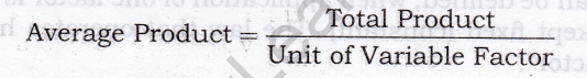
2.Average product or Average return to an input: It is per unit total product of variable factors. It is calculated by dividing the total Product by the units of variable factor.
3. Marginal Product or Marginal Return to an Input: It is an addition to the total product when an additional unit of a variable factor is employed.
4. Total Product, Average Product and Marginal Product with the help of schedule and diagram are as follows:
Explanation of a Curves
1. TP increases continuously from points O to A. It increases at an increasing rate (convex shape) from O to P and at a diminishing rate (concave shape) from P to A. TP is maximum at A and remains so upto point B. After point B, Total product falls.
2. MP curve initially rises, reaches its maximum and ultimately declines taking the shape of inverted U.
3. Similarly, AP curve first rises, reaches its maximum and then declines taking the shape of an inverted U.
4. Return to a variable factor states that change in the physical output of a good when only the quantity of one input is increased, while that of other input is kept constant.
Law Of Variable Proportions
1. The law of variable proportion states that as we increase the quantity of only one input, keeping other inputs fixed, the total product increases at an increasing rate (convex shape) in the beginning, then increases at diminishing rate (concave shape) and after a level of output ultimately falls.
2. Assumptions of Law of Variable Proportions
(a) Only one input is variable, the other is held constant or fixed.
(b) It is possible to change the proportion in which the factor units are combined.
(c) It assumes a short run.
(d) The state of technology is given and remains unchanged.
(e) Price of factors of production do not change.
3. It can be explained with the help of schedule and diagram:
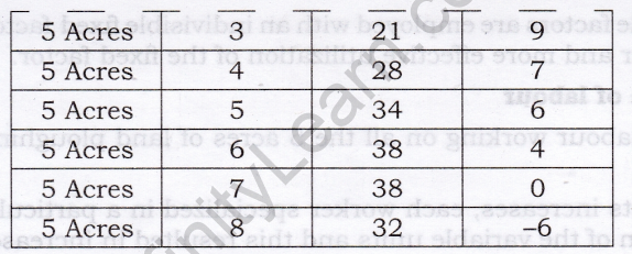
4. Explanation of Each Phase
Phase I: Phase of increasing return or Increasing Return to factor
(a) It is called the stage of increasing returns.
(b) The total product increases at an increasing rate (convex shape) up to point P. The marginal physical product of labour (MP) is increasing and reaches its highest point Pp vertically downwards to point P.
(c) Point P is called the point of inflexion. At point P, the curvature of the TPP curve changes. It stops increasing at an increasing rate and starts to increase at a diminishing rate.
In the first stage, firm is moving towards achievement of ideal combination of factors in which TP is increasing at an increasing rate at every level of output. So, instead of stopping its production, the firm will rather continue employing additional units of a variable factor.
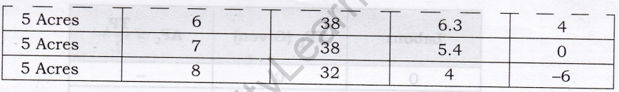
Phase II: Stage of Diminishing Returns or Diminishing Return to factor
(a) The total product (TP) continues to increase, but at a diminishing rate (concave shape) and eventually becomes the highest.
(b) MP is diminishing but is positive.
(c) The stage comes to an end, when Marginal Product (MP) = 0 and Total Product (TP) is maximum and constant.
The firm would like to operate in the second phase because TP is maximum and there is proper utilization of fixed factor.
Phase III: Phase of Negative returns or Negative Return to factor
(a) In this stage the total product declines in absolute terms.
(b) The marginal product becomes negative.
The firm cannot operate in the third stage where MP is negative and TP starts declining as we are moving beyond the optimum degree of specialisation.
5. There are 3 important reasons or causes for the operation of increasing returns—
(a) Proper utilization of the fixed factor
(i) In the initial stage of production the units of variable input i.e., labour) is so less that fixed inputs cannot be effectively utilized.
(ii) Proper utilization of the fixed factor can be attained when more and more units of variable factor (labour units) are applied to the fixed factor (land), the fixed factor will be used intensively and output will increase rapidly.
(b) Indivisibility of fixed factor
(i) Indivisibility of fixed factor means that due to technological requirements a minimum amount of fixed factor must be employed, whatever the level of output,
i.e., fixed factor cannot be divided into smaller units.
(ii) Thus, as more units of variable factors are employed with an indivisible fixed factor, output increases due to fuller and more effective utilization of the fixed factor.
(c) Specialization and division of labour
(i) Initially there was only one labour working on all the 5 acres of land ploughing, watering, etc.
(ii) As the number of labour units increases, each worker specialized in a particular activity leads to specialization of the variable units and this resulted in increased output.
6. Reasons for diminishing returns:
(a) The non-optima! combination of variable factor with the fixed factor
(i) When a given quantity of a fixed factor is combined with more and more units of variable factor, the additional units of variable factor will have smaller and smaller quantity of fixed factor to work with them.
(ii) As many workers share the same fixed factor, the share of each would obviously fall. Therefore, the cooperation of the fixed factor is not available to the same extent. Thus, an increase in the variable factor would add less and less to total output.
(b) Imperfect Substitutes
(i) Diminishing return to factor occurs because variable factor and fixed factor are imperfect substitutes to each other.
(ii) Technically speaking, there is a limit to which variable factor can be applied to fixed factor and that limit depends upon the efficiency of fixed factor. So, variable factor and fixed factor are imperfect substitutes to each other.
7. Reasons for Negative returns:
(a) Scarcity of Fixed Factor
(i) During a short period, there is a limitation that we cannot change the fixed factor.
(ii) So, variable factor can be change upto a certain limit and that limit depends upon the efficiency of fixed factor. If we cross that limit, the total product starts falling.
(b) Efficiency of Variable Factor Fall
(i) In this stage the amount of variable factor becomes excessive relative to the fixed factor. This happens when too many LABOUR are engaged in cultivating on a given piece of land.
(ii) Instead of helping each other in production they cause overcrowding and chaos and thus hamper each other’s work. In such a case, the contribution of additional labour to production is bound to be negative.
(iii) Thus, the marginal returns become negative and the total returns start diminishing.
(c) Efficiency of Fixed Factor Fall
(i) Too much of a variable factors may also lead to the inefficiency of the fixed factor as well.
(ii) In case of machine, which is a fixed factor, too much of labour may cause lot of wear and tear of machinery, frequent breakdowns and excessive cost of maintenance. This is bound to affect total production adversely.
(iii) In such a situation it is advisable to reduce the units of the variable factor than to increase it with a view for getting maximum production.
Law Of Diminishing Marginal Returns
1. The Law of diminishing marginal return states that when we applied more and more units of variable factor to a given quantity of fixed factor, total product increases at a diminishing rate and marginal product falls.
2. Law of diminishing marginal returns is a classical theory and classical economists treated it as a separate Law. But according to modern economists, this law indicates just one aspect (aspect of diminishing returns) of law of variable proportion.
3.
In the above schedule and diagram when more units of variable factor are employed with a given quantity of fixed factor TP increases at a diminishing rate or MP goes on falling. That is why shape of MP curve is a downward sloping.
Words that flatter
1. Production function: The relationship between physical input and physical output of a firm is generally referred to as production function.
The general form of production function is,
q = f ( x1 ,x2)
where, q = output, x1 = 1 input like labour, x2 = another input like machinery
2. Variable factors: It refer to those factors, which can be changed in the short run. They vary directly with the output. For example, Labour, raw material, etc.
3. Fixed factors: It refer to those factors which cannot be changed in the short run. They do not vary directly with the output. For example, Capital, land, plant and machinery, etc.
4. Short period: It refers to the period of time in which a firm cannot change some of its factors like plant, machinery, building, etc. due to insufficiency of time but can change any variable factor like labour, raw material, etc.
5. Long period: It refers to a time period during which a firm can change all its factors of production including machines, building, organization, etc.
6. Total product: It refers to total volume of goods and services produced by a firm with the given input during a specified period of time.
7. Average product: It is per unit product of variable factors. It is calculated by dividing the total Product by the units of variable factor.
Average Product=Total Product/Unit of Variable Factor
8. Marginal Product: It is an addition to the total product when an additional unit of a variable factor is employed.
MP=Change in output /Change in input =Δq/ΔL
9. Return to a factor: It states that change in the total output of a good when only the quantity of one input is increased, while that of other input is kept constant.
10. Law of variable proportion: It states that as we increase the quantity of only one input, keeping other inputs fixed, the total product increases at an increasing rate in the beginning, then increases at diminishing rate and after a level of output ultimately falls.
11. Law of diminishing marginal return: It states that when we applied more and more units of variable factor to a given quantity of fixed factor, total product increases at a diminishing rate and marginal product falls.